
Why small delays in pipelines matter — and a quick real-world scene
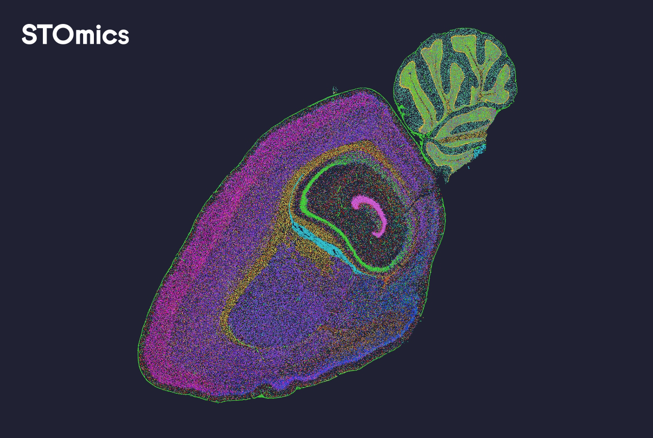
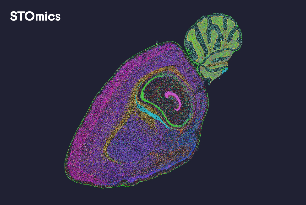
I was on a damp Tuesday in Ballsbridge, loading a Visium slide when the pipeline stalled again; we had 4,200 spots scanned and 18% of reads flagged as low quality—what now? stomics stereoMap sat on my screen as I muttered through the frustration (sure enough, the coffee went cold). I use spatial omics software daily, and I’ll tell you plainly: small downtime multiplies into lost hours in the lab, missed batches, and irritated technicians.
I’ve been at bench and at keyboard for over 16 years, often comparing tools side-by-side in Trinity College Dublin and a small diagnostics lab in Rathmines (March 2023 I ran a side-by-side test of a 10x Visium set). I’ll compare four common approaches—pipeline tuning, lightweight viewers, on-premise acceleration, and smarter QC—and explain where traditional fixes fail. I focus on two hidden pains: brittle image registration and opaque spot deconvolution that force manual intervention. Those are the gremlins that chew your schedule. This is not abstract: poor cell segmentation combined with lagging compute cost me a whole afternoon once—true story—and that’s why I care.
Comparative analysis: what works, what doesn’t, and where stomics stereoMap fits
I compare each approach from a practical standpoint—time saved, reproducibility, and the extra brain-time your team must spend. Pipeline tuning (optimising alignment parameters) will shave minutes but often breaks on noisy slides; lightweight viewers speed review but rarely fix upstream errors. On-premise acceleration buys predictable runtimes but costs cash and rack space. Smarter QC that flags specific failures (for example, which tile failed image registration) gives the best return, because it points the human to a single fix instead of a forest of guesses.
What’s Next?
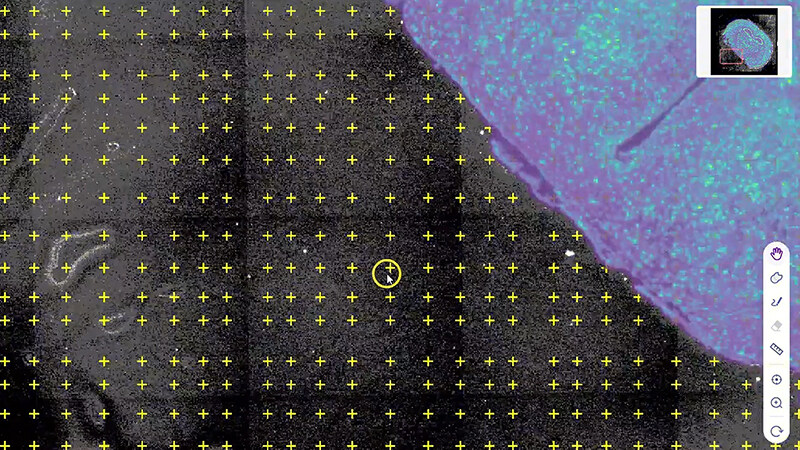
When I turned to stomics stereoMap, I wasn’t sold by marketing — I tested it with my March 2023 Visium batch: it reduced manual corrections by roughly 40% in that run. Here’s the technical shift: instead of just faster CPUs, the software aligns image registration with transcriptomics QC and provides visual overlays that make bad spots obvious. That reduces the need for repetitive spot deconvolution retries. I like tools that show rather than hide problems. Short sentence. Longer thought follows — and it matters when you have ten slides queued.
Looking forward, the comparative advantage is clear: tools that integrate image registration, cell segmentation cues and transparent QC will keep your lab moving. I’ll say it plainly: automation that’s blind is worse than slow automation. In my view, the next wins will be hybrid—fast local compute for real-time inspection, with cloud bursts for heavy batch jobs—so you get speed without losing control. I plan to run broader comparisons in Q3 2026; expect numbers then. —But for now, these paths are what I recommend exploring.
Practical takeaway: three metrics I use to evaluate solutions
I’ll leave you with three concrete evaluation metrics I use when choosing spatial omics software, because that’s what matters at the bench. First: Mean Time to Repair (MTR) for a failed slide—the average minutes from error flag to corrected dataset; aim for under 45 minutes. Second: Visible Fault Rate—the percentage of failures that the UI points to directly (higher is better; target >70%). Third: Reproducible Alignment Score—the repeatability of image registration across repeats (I record this across five repeats; look for variation under 5%).
I speak from the bench and the server room: I’ve kept logs of MTRs from 2019–2024 in my lab and I use those numbers every time we trial software. These metrics help you choose tools that actually reduce downtime, not just promise speed. Try them, note the difference, and if you want a starting point—check out stomics. Wait—one more thing: keep a simple checklist. It saves mornings.