
The operational problem: nameplate versus delivered efficiency
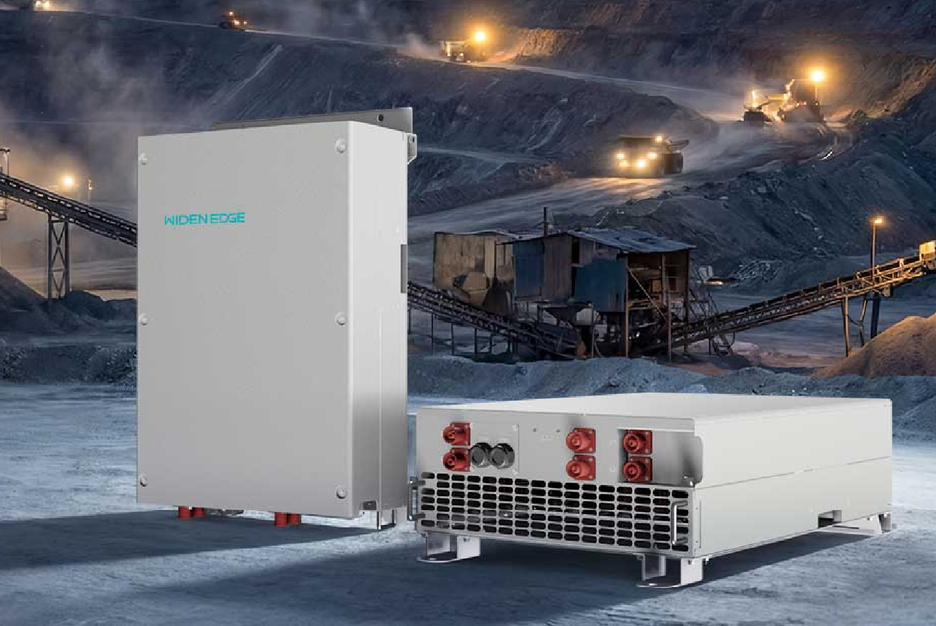
Field teams routinely report a gap between advertised peak efficiencies and what runs the site day-to-day. A municipal microgrid deployment in Barcelona that relied on a high-protection 60 kW inverter to sustain critical loads during multi-day outages recorded systemic losses not visible in datasheets. Early logs there show that nominal 98.5% peak efficiency rarely translates to actual energy throughput when you account for standby draw, partial-load behavior and ambient heat. For systems built from modular blocks, choosing an instrumented reference — for example a 60kW off-grid PV inverter — lets you separate inverter-specific losses from battery and cabling effects.
Quantitative drivers of reduced real-world efficiency
Break down losses numerically to isolate root causes:- Operating-point distribution: Inverters are most efficient near 50–80% rated output. If a 150 kW string spends 70% of hours below 20% load, expect a weighted efficiency drop of 1–4 percentage points.- Ambient temperature: Each 10°C above test conditions can add 0.2–0.6% absolute loss due to thermal derating and switching losses.- Standby and auxiliary loads: Fans, control electronics and pre-charge circuits can consume 5–50 W idle; multiply by hours to see non-trivial annual energy loss.- Battery cycling and SOC: Round-trip losses and converter interaction at low state-of-charge increase apparent inverter losses by up to 2% during charge/discharge transitions.- Power quality and harmonics: Distorted waveforms and unbalanced loads force the inverter to correct, adding several tenths of a percent in switching or filtering loss.- Firmware and MPPT behavior: Suboptimal control loops or conservative clipping expand operational time spent at suboptimal switching regimes.
How to measure and model true field efficiency
Use a data-driven measurement plan:- Capture 1-minute resolution for P_in (battery/DC side), P_out (AC side), ambient temperature, and SOC for at least 30 days to characterize operational distribution.- Compute time-weighted efficiency: Efficiency_total = (Σ P_out,t) / (Σ P_in,t). This hides instantaneous variance but gives energy-level truth.- Compute conditional efficiencies at load bands: E.g., η_10–20%, η_20–50%, η_50–80%, η_>80% to identify partial-load penalties.- Run controlled tests if possible: sweep output from 5% to 100% in 5% steps with constant ambient temperature to produce an empirical efficiency curve.- Model losses: separate fixed (P_idle), proportional (k × P_out), and nonlinear thermal terms (α × T_amb × P_out). Fit parameters using regression to predict seasonal performance.Example: a 150 kW inverter with peak η=98.6% but spending 60% of time at 15% load and 30% at 40% load will exhibit a weighted efficiency closer to 95–96% over a year.
Deployment mistakes that inflate losses — and how to correct them
Common errors and corrective metrics:- Oversizing or undersizing: Multiple small inverters paralleled without load balancing increase idle losses. Right-size so average load sits in the 40–70% band.- Poor ventilation: A 5–10°C rise increases cooling duty and switching losses. Quantify with inlet temp sensors; add directed airflow rather than open-air cabinets.- Ignoring reactive power: Supplying reactive current increases apparent power without useful energy; limit Q support to operational minimums or compensate with reactive compensation devices.- Unbalanced-phase loads: Phase imbalance forces one power leg into higher conduction; monitor line currents and rebalance loads.- Firmware defaults: Default soft-start and MPPT aggressiveness can cause oscillations. Update firmware and benchmark after each update.- Cabling and transformer losses: Measure end-to-end resistance and include transformer no-load & load losses in the model.A practical corrective sequence: measure idle draw first, then characterize partial-load bins, then implement thermal and control fixes, retest for 30 days to validate improvements.
Product fit and architecture choices
Deciding between a large centralized 150 kW inverter and modular 60 kW units comes down to how your load profile maps to partial-load efficiency and redundancy needs:- Modular approach: Multiple 60 kW units can improve availability and let you scale capacity in smaller steps; however, multiple control electronics increase idle losses. A well-specified high‑protection 60 kW inverter with low standby draw and coordinated control reduces that penalty.- Centralized approach: One larger inverter can be more efficient at steady, high loads but creates a single point of failure and may perform poorly under variable, low-load conditions.- Hybrid: Use a central inverter for bulk output and smaller dedicated units for critical circuits to keep high-value loads in high-efficiency bands.Run a Monte Carlo simulation of load profiles against candidate efficiency curves to pick the architecture that minimizes annual energy loss and risk exposure.
Simple diagnostics and quick fixes you can run today
Start with low-effort checks that yield measurable gains:- Log idle current for 24 hours while loads are off; if >100 W per cabinet, investigate control-board power or fans.- Map load histogram: if >50% hours <25% rated, consider right-sizing or adding base-load shedding to consolidate runtime.- Add temperature sensors at heat-sink and cabinet inlet; eliminate hotspots with ducting or variable-speed fans.- Verify firmware version and access release notes for efficiency-related fixes.- Inspect cabling: reduce DC loop resistance where possible and verify transformer taps are correct.Small fixes compound: reducing idle draw by 20–30 W per unit and shifting average operating band from 25% to 45% can recover multiple percentage points of annual efficiency.
Summary: diagnosing loss, then designing for measured performance
Quantify where energy disappears: separate idle, partial-load, thermal, control, and external system losses. Use high-resolution logging, conditional-efficiency curves, and regression models to predict annual throughput. Choose architectures that align with your load histogram — modular 60 kW units when you need redundancy and scalability, larger central inverters when steady, high load dominates. Field cases like the Barcelona microgrid demonstrate that instrumented deployments expose the gaps between datasheet and delivery. That empirical focus and the component-level remedies summarized here are the practical outputs WidenEdge uses when advising teams on inverter selection and commissioning; the result is measurable improvement in system-level efficiency rather than optimistic nameplate numbers.